
DCW: Solving the SNR-t Bias for High-Fidelity Diffusion Sampling
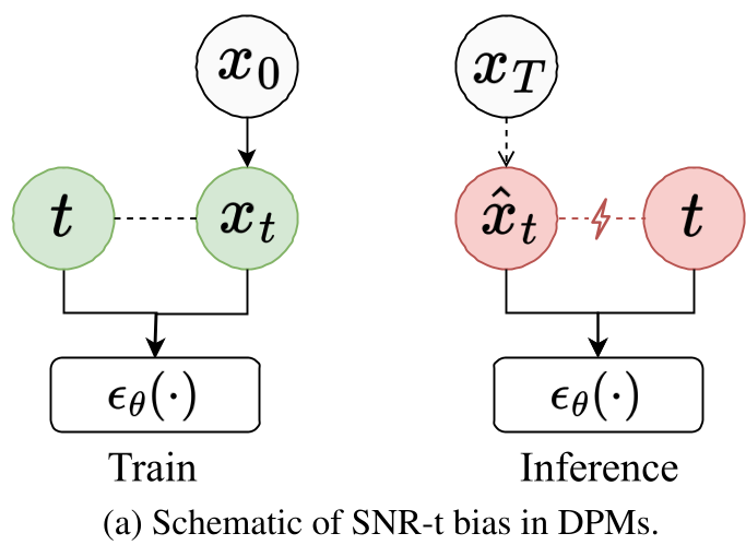
Elucidating the SNR-t Bias of Diffusion Probabilistic Models
The paper identifies and investigates the "SNR-t bias" in Diffusion Probabilistic Models (DPMs), proposing a plug-and-play method called Differential Correction in the Wavelet domain (DCW). This training-free approach mitigates the misalignment between sample signal-to-noise ratio and timesteps, significantly improving generation quality across various SOTA models including FLUX and EDM.
TL;DR
Diffusion models are built on a fragile promise: that the noise level (SNR) of a sample will always match its assigned timestep (t). This paper reveals that this promise is systematically broken during inference—a phenomenon called SNR-t Bias. By introducing Differential Correction in the Wavelet domain (DCW), the authors provide a training-free, "plug-and-play" fix that drastically reduces FID scores (up to 47%) with almost zero computational cost.
The Hidden Flaw: Why Your Diffusion Model Overestimates Noise
In the training phase of a Diffusion Probabilistic Model (DPM), the relationship between the Signal-to-Noise Ratio (SNR) and the timestep is deterministic. The model learns to denoise based on this strict coupling.
However, the authors discovered a critical discrepancy during inference. Due to discretization errors from solvers and residual prediction errors from the network, the reverse denoising trajectory drifts. Specifically:
- Key Finding 1: Models are highly sensitive to SNR-t mismatch. If the input sample has a lower SNR than expected for that timestep, the network overestimates the noise.
- Key Finding 2: Reverse process samples consistently exhibit lower SNR than their forward-process counterparts at the same .
This creates a vicious cycle of error accumulation, leading to images that appear over-smoothed, overexposed, or structurally incoherent.
 Above: Evidence showing that reverse noise predictions consistently overestimate compared to the ideal forward process.
Methodology: Differential Correction in the Wavelet Domain
The authors suggest that if we can push the biased predicted sample back toward the "ideal" perturbed distribution, we can neutralize the bias.
1. The Gradient Intuition
The core of the solution lies in the Differential Signal. By taking the difference between the current predicted sample and the reconstructed clean sample , the model implicitly gains a "gradient" that points back toward the ideal trajectory.
2. Why Wavelets?
Instead of applying this correction uniformly across pixels, DCW decomposes the image using a Discrete Wavelet Transform (DWT) into:
- Low-frequency (LL): Global structures and contours.
- High-frequency (LH, HL, HH): Fine textures and details.
This aligns with how DPMs work: they build the house (low-freq) before painting the windows (high-freq). DCW uses a Dynamic Weighting Strategy:
- Early Stage: High weight on low-frequency correction to secure global structure.
- Late Stage: High weight on high-frequency correction to ensure crisp details.
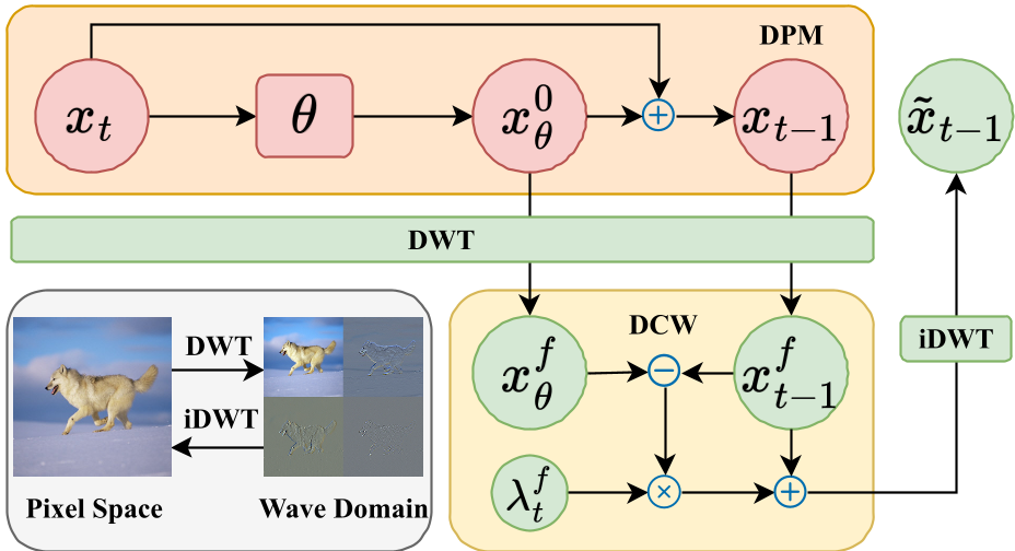 The DCW Pipeline: Decomposing the signal, applying frequency-specific correction, and reconstructing via iDWT.
Experimental Performance
The results are strikingly consistent across resolutions and architectures.
- On EDM: FID dropped from 10.66 to 5.67 (a ~47% improvement) in 13-step sampling.
- On FLUX: Qualitative results show significant reductions in overexposure and blurring, yielding "aesthetic" improvements that are immediately visible to the human eye.
- Efficiency: Because DWT and iDWT are computationally cheap and the correction utilizes existing network outputs, the overhead is less than 0.5%.
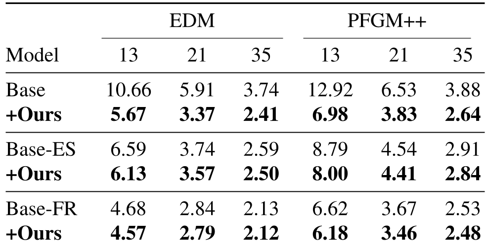 Comparison on EDM and PFGM++ architectures showing consistent FID reduction.
Critical Insight & Conclusion
This work shifts the focus from "Exposure Bias" (which looks at data distribution) to "SNR-t Bias" (which looks at structural coupling). By providing a rigorous mathematical proof (Theorem 5.1) that the reverse SNR is always lower than the forward SNR, the authors have diagnosed a fundamental illness in diffusion sampling.
Takeaway: DCW is a rare "free lunch" in deep learning. It requires no retraining, works on almost any DPM variant, and addresses a core theoretical flaw that has plagued high-speed sampling since the inception of DDIM.
Limitations
While DCW is robust, it relies on hyperparameter tuning for (the guidance factor). Although the authors demonstrate a simple search strategy, an automated, parameter-free version of this correction would be the natural next step for the community.