
Constrained Spectral Preconditioning: The Theoretical Bridge Between Muon and Hard Constraints
Constrained Stochastic Spectral Preconditioning Converges for Nonconvex Objectives
This paper introduces a unified framework for proximal preconditioned gradient methods, specifically extending spectral optimizers like Muon and Scion to handle both convex and nonconvex constraints. The authors propose a family of stochastic algorithms that utilize a novel "anisotropic proximity operator" and prove convergence under heavy-tailed noise, achieving SOTA results in constrained neural network training tasks such as transformer "grokking" and NanoGPT.
TL;DR
Spectral optimizers like Muon and Scion have taken the AI world by storm by updating weights using the matrix sign of the gradient rather than the raw gradient itself. However, these methods usually ignore "hard" constraints (e.g., keeping weights on a sphere). This paper introduces a proximal spectral preconditioning framework that allows these SOTA optimizers to handle nonconvex constraints (like the Stiefel manifold) with rigorous convergence proofs, even in the presence of heavy-tailed noise.
The "Broken" Proximal Step
In standard SGD, if you have a constraint (like ), you just project the parameter back after each step. But in spectral methods, the update direction (from the SVD of the gradient) changes the geometry. If you use a standard Euclidean projection, the algorithm might stop at a point that isn't actually a minimum of your loss function.
The authors solve this by using an anisotropic proximal operator. Instead of checking "is this point close in Euclidean distance?", it checks "is this point close according to the geometry of the spectral preconditioner?".
Methodology: Singular Value Geometry
The core insight is that for modern neural network layers (2D weights), the most effective constraints are orthogonal invariant—they only care about the singular values, not the specific orientation of the weight matrix.
1. Forward Step (Adaptive Update)
The algorithm first takes a step in the dual space:
abla \phi^*(d^k)$$ Where $\phi^*$ is the convex conjugate of a reference function that defines the "spectral" behavior (like the matrix sign). ### 2. Backward Step (The Constraint) It then solves a proximal subproblem: $$x^{k+1} = ext{arg min } g(x) + (\gamma_k \star \phi)(x - y^k)$$ By leveraging **Theorem 3.5**, the authors show that even for complex matrix constraints (like the Stiefel manifold or Spectral balls), you can simply perform the SVD, apply the constraint to the **singular values** (a 1D operation), and reconstruct the matrix. 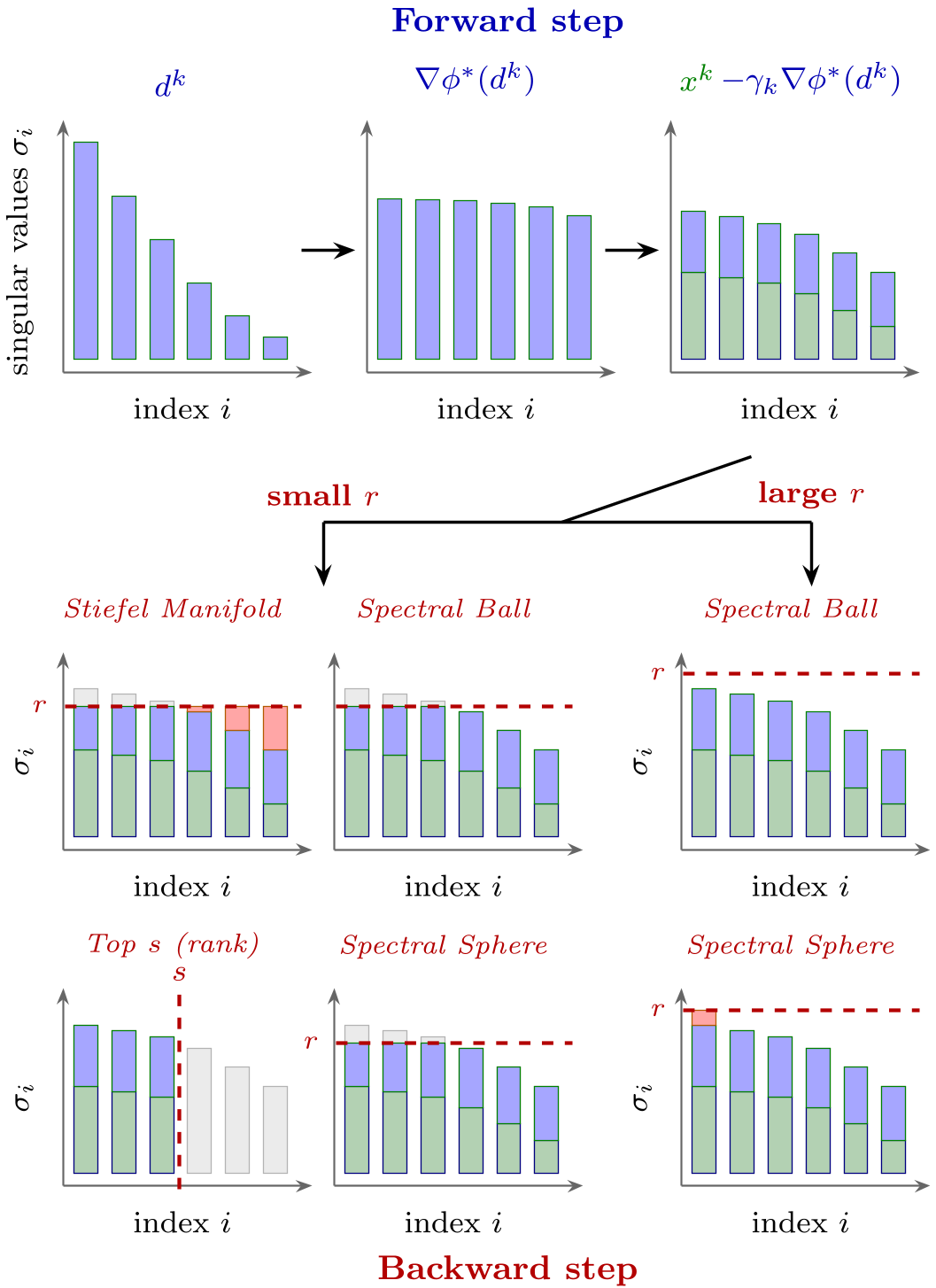 *Caption: Visualization of how different spectral reference functions $\phi$ reshape the optimization landscape and projection steps.* ## Handling the Noise: Storm and Heavy Tails Deep learning gradients are notoriously "noisy" and often follow heavy-tailed distributions. This paper proves that preconditioned methods are naturally robust to these outliers. By integrating the **STORM (STochastic Recursive Momentum)** estimator, they achieve faster variance reduction without requiring massive batch sizes. ## Experimental Highlights - **Accelerating Grokking**: On modular arithmetic tasks (DivMod97), enforcing spectral norm constraints through this framework significantly reduced the number of epochs required for the model to "grok" (generalize from training to validation set). - **NanoGPT (124M)**: Using a Frobenius ball constraint on spectral layers led to more stable and faster training compared to unconstrained Scion baselines. 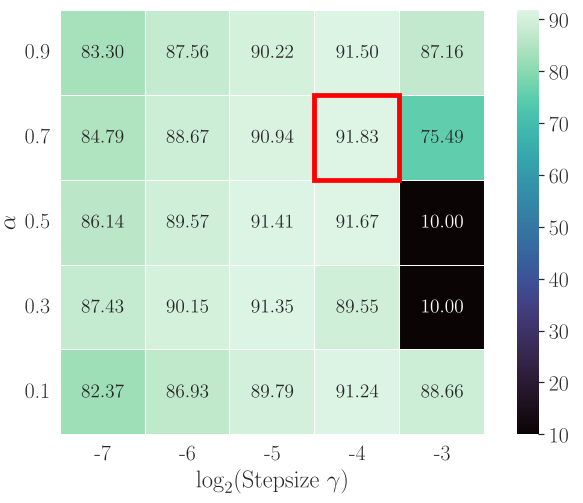 *Caption: Comparison of training epochs to reach 95% accuracy. Hard constraints (right) show more consistent generalization across different parameter scales.* ## Conclusion & Future Outlook This work moves us closer to a "unified theory of optimization" where weight decay, gradient clipping, and spectral updates are all seen as specific instances of **anisotropic proximal gradients**. **Limitations**: The primary bottleneck remains the computational cost of the SVD required for the proximal step. While the authors use "Polar Express" (polynomial approximations) to speed this up, calculating exact projections for every layer in a 70B parameter model is still a challenge for the future. **Takeaway**: If you want your transformer to generalize faster, don't just decay the weights—constrain their singular values.