Beyond Precise Timestamps: Managing Uncertainty with Interval-Based Timing Constraints

    ## TL;DR
    In the world of real-time distributed systems, "exactly at time $t$" is a myth. This paper proposes a transition from binary point-based constraints to probabilistic **Interval-Based Timing Constraints**. By modeling event occurrences as non-uniform distributions (like Exponential or Normal), the researchers provide a mathematical toolkit to calculate the probability of satisfying a deadline and an algorithm to root out hidden (implicit) constraints.

    ## Background: The Death of Deterministic Timing
    In classical real-time theory, we assume we know exactly when an event occurs. However, in modern networked and embedded systems, software execution time is jittery. If we can't pinpoint the time, we use an **Interval Timestamp** $I = [\min, \max]$. 

    But once you move to intervals, "Did the deadline pass?" is no longer a Yes/No question. It becomes a probability. The core contribution of this work is moving beyond the "uniform distribution" assumption found in earlier research to handle more realistic, non-uniform scenarios like transient hardware faults.

    ## Methodology: The Math of Confidence
    The authors define a timing constraint not just as a duration $d$, but as a tuple $\langle d, P \rangle$, where $P$ is the **Confidence Threshold**.

    ### 1. Satisfaction Probability (SP)
    To determine if a constraint $I_2 - I_1 \leq d$ is satisfied, the authors integrate the joint density function of two independent events over the satisfiable region (where $y \leq x + d$). 

    ![Joint Density Function Mapping](https://cdn.atominnolab.com/wisdoc/images/20260604-ed4c1287-815c-42dc-ac74-7b82db565182/page_002_block_002.png)
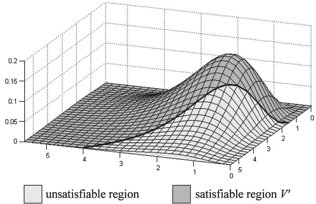
    *Fig 1: The dark-shaded region represents the satisfiable area under a specific distribution.*

    ### 2. Deriving Implicit Constraints
    A system of constraints often hides more "stringent" requirements. For example, if $A 	o B$ is 5ms and $B 	o C$ is 5ms, then $A 	o C$ is implicitly 10ms. For interval constraints, the authors developed an $O(n^3)$ algorithm based on the Floyd-Warshall approach. 
    *   **Time Domain**: Paths are combined using *Min-Plus* algebra (finding the shortest path).
    *   **Confidence Domain**: Paths are combined using *Max-Product* algebra (finding the highest probability).

    ## Analytical Insights: The 50% Rule
    One of the most powerful "PhD-level" insights in the paper is the discovery of bounds. For certain configurations (specifically the $\pi\delta$ configuration), the authors prove that:
    
    > **Theorem**: If events follow an Exponential or Normal distribution, the maximum possible Satisfaction Probability (SP) is only **50%**.

    This is a massive win for system designers. If a requirement demands a 90% confidence threshold ($P=0.9$) for a setup that is mathematically capped at 50%, the system is **intrinsically unsatisfiable**. You can solve the problem at compile-time without ever running a single line of code.

    ## Applications: Fault Monitoring and Voting
    The paper proves its worth in two messy, real-world scenarios:
    
    1.  **Distributed Fault Monitoring**: Modeling transient faults as Poisson arrivals. The math helps determine if a system can actually meet fault-tolerance guarantees given recovery times.
    2.  **Composite Event Voting**: In a "k-out-of-n" sensor voting scheme, the time to reach a consensus is a "composite event." Even if individual sensors are uniform, the group behavior is non-uniform.

    ![Experimental Parameter Plot](https://cdn.atominnolab.com/wisdoc/images/20260604-ed4c1287-815c-42dc-ac74-7b82db565182/page_013_block_002.png)
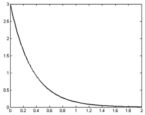
    *Fig 2: Calculating satisfaction probabilities for consistency constraints in a dual-sensor (IR and RW) environment.*

    ## Critical Analysis & Takeaways
    The beauty of this work lies in its **Heuristic Insight**: treating timing as a resource with a risk profile rather than a hard boundary.
    
    *   **Advantages**: It allows for "intelligent risk-taking." If a point-based solution says "Impossible," this model says "It's possible with 85% confidence if you add two more sensors."
    *   **Limitations**: The model assumes independent event occurrences ($f(x)$ and $g(y)$). In many distributed systems, events are temporally correlated (causally linked), which would require more complex conditional density functions.
    *   **Future Impact**: This sets the stage for "Adaptive QoS" in middleware, where a system can reallocate resources the moment the *probability* of a violation creeps too high, rather than waiting for the violation to actually occur.

    ## Summary
    By formalizing the "satisfaction probability" of timing constraints, Yu et al. have provided a bridge between rigid real-time theory and the messy, uncertain reality of distributed hardware.