The Geometry of Chaos: Decoding the Origin of the Edge of Stability

Executive Summary

TL;DR: Gradient Descent (GD) in deep learning has a "speed limit." When training, the sharpness of the loss landscape (the largest Hessian eigenvalue ${\lambda }_{max}$) typically rises until it hits exactly $2/\eta$ (where $\eta$ is the learning rate). At this point, training doesn't fail; it enters the Edge of Stability (EoS), characterized by oscillations and non-monotonic loss decrease. This paper provides a unified global theory using a novel "edge coupling" functional to prove that EoS is a fundamental attractor of the discrete dynamical system.

Background Location: This work moves EoS theory from local observations (what happens at the edge) to a global "conservation law" (why the system is forced to the edge). It bridges classical optimization with discrete Hamiltonian mechanics.

The Problem: Why Does 2/η Rule Everything?

In classical optimization theory, we are taught that training is stable only if $\eta <2/{\lambda }_{max}$. However, modern neural networks routinely violate this. Cohen et al. (2021) observed that ${\lambda }_{max}$ actually climbs up to $2/\eta$ and oscillates there.

Previous attempts to explain this were "local"—they showed that if you are already near $2/\eta$, the dynamics might keep you there. But they couldn't explain why a trajectory starting far away would inevitably find its way to this specific threshold.

Methodology: The Edge Coupling

The author's brilliant insight is to treat gradient descent iterates not just as a sequence, but as critical points of a specific functional called the edge coupling:

${\mathcal{A}}_{\eta }(x,y)riangleqL(x)+L(y)-\frac{1}{2\eta }\Vert x-y{\Vert }_2^2$

The Intuition:

1. Stationary Edges: If you set the gradient of ${\mathcal{A}}_{\eta }$ with respect to $x$ to zero, you exactly recover the Gradient Descent update formula.
2. The "Spring" Analogy: The term $-\frac{1}{2\eta }\Vert x-y{\Vert }^2$ acts like a negative spring constant. It represents the "energy" of the step.
3. Period-Two Orbits: When both $x$ and $y$ are critical, the system describes a state where the model bounces back and forth between two points—the hallmark of EoS behavior.

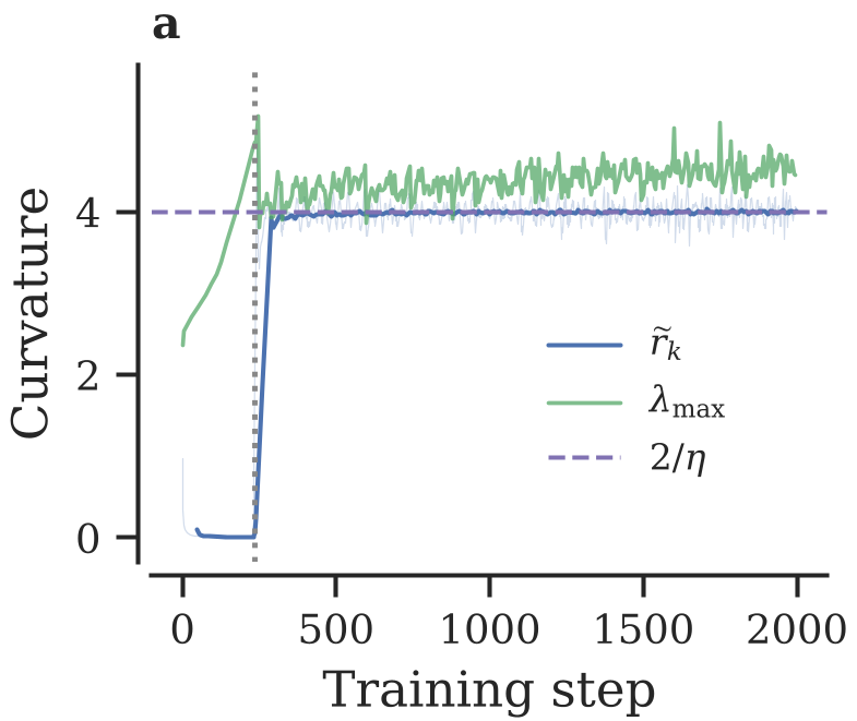Figure 1: Evolution of effective curvature and sharpness. Note how they saturate exactly at the dashed 2/η line.

The Core Results: Forcing and Localization

The paper’s most significant contribution is the Curvature Concentration Theorem. By summing the one-step loss changes, the author derives a telescoping sum:

${\sum }_{k=0}^{K-1}\Vert d_k{\Vert }_2^2\left(\frac{2}{\eta }-{\tilde{r}}_k\right)=2(L(w_0)-L(w_K))$

Why this matters: Since the total loss drop ($L(w_0)-L(w_K)$) is finite, but the steps $\Vert d_k{\Vert }^2$ keep accumulating, the term in the parenthesis $(\frac{2}{\eta }-{\tilde{r}}_k)$ must approach zero. Mathematically, the trajectory is "forced" to visit regions where the curvature ${\tilde{r}}_k\approx 2/\eta$.

Furthermore, using the Mean Value Theorem, the paper proves that there exists a point exactly on the line between two iterates where the true Hessian eigenvalue is $\ge 2/\eta$. No approximations, no gaps—just pure geometric necessity.

Bifurcation in Linear Networks

To test the theory, the author analyzed two-layer linear networks. They found:

• Width Invariance: The stability of the "Edge" doesn't change whether your hidden layer has 100 neurons or 10,000. Overparameterization just adds "flat" directions but doesn't move the 2/η boundary.
• The Pitchfork: As $\eta$ crosses the critical threshold ${\eta }_c$, the stable fixed point "splits" into a period-two orbit. This is a classic pitchfork bifurcation confirmed by experimental data.

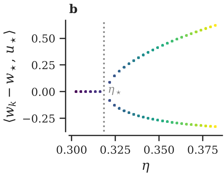Figure 2: Pitchfork diagram showing the continuous emergence of oscillations as η exceeds the critical threshold.

Deep Insights: Stability Mechanisms

Why doesn't the model just blow up when it hits the Edge of Stability? The paper identifies two regimes:

1. Growth above threshold: If curvature exceeds $2/\eta$, the step sizes grow exponentially, which quickly pushes the model into a different region of the landscape.
2. Oscillatory Cancellation: Inside the "Edge" phase, the steps alternate signs. Even if the multipliers are near -1, the oscillations effectively cancel each other out, preventing the weights from drifting to infinity.

Conclusion & Future Outlook

Elon Litman’s work provides the "Missing Link" in optimization theory for deep learning. It proves that the Edge of Stability isn't a bug; it's a feature of how discrete steps interact with loss surfaces.

Limitations: The theory currently requires smooth ($C^2$ or $C^4$) loss functions, which technically excludes raw ReLU activations (though smoothed ReLUs fit perfectly).

What's Next?: The next frontier is applying this "edge coupling" framework to Stochastic Gradient Descent (SGD) and adaptive methods like Adam, which may explain why large-batch training often feels "sharper" and more unstable than small-batch training.

Takeaway for Practitioners: When you see your loss curve start to jitter/oscillate, you haven't necessarily chosen a "bad" learning rate. You've simply reached the Edge of Stability, where the model is actively regularizing its own sharpness to stay on the 2/η boundary.