ASPO: Navigating the Hurdles of Mobile Social Networks through Improved A-Star

    ## TL;DR
    Finding the "shortest path" in a digital map is easy; finding it in a messy, real-world Mobile Social Network (MSN) filled with temporary obstacles is much harder. This paper introduces **ASPO (A-star Shortest Path with Obstacles)**, an approach that optimizes the A-star algorithm to bypass obstructions while maintaining the low latency required for Location-Based Services (LBS).

    ## Problem & Motivation: The Reality of Obstacles
    Most pathfinding research operates under the "ideal world" assumption—that the shortest distance between two points is a static line. However, in MSNs, reality is dynamic. Road construction, temporary closures, and traffic accidents change the graph topology in real-time. 

    Prior work often suffers from two extremes:
    1. **Ignoring Obstacles**: Leading to paths that are physically short but practically impossible.
    2. **High Latency**: In large-scale graphs (millions of nodes), exhaustive searching to avoid obstacles becomes too slow for mobile users who expect instant results.

    The authors' insight is to modify the **A-Star algorithm**—the gold standard for graphic search—to specifically handle these constraints by dynamically updating the directed edge set $E$.

    ## Methodology: The Improved A-Star Model
    The core of the ASPO approach lies in its refined evaluation function. Traditionally, A-star uses $f(n) = g(n) + h(n)$, where $g(n)$ is the cost from the start and $h(n)$ is the heuristic estimate to the goal.

    ### 1. The Heuristic Formula
    The authors enhance the heuristic $h(n)$ by introducing an adjustable Manhattan distance:
    $$h(n) = d(v_c, v_d, \alpha, \beta) + d'(V_c, v_d, \alpha, \beta)$$
    - **$\alpha$ and $\beta$**: These are adjustment parameters (where $\alpha + \beta = 1$) that allow the algorithm to weigh horizontal vs. vertical movement based on the grid structure.
    - **Historical Context ($d'$)**: It considers the average distance of previous vertices on the path, providing a "smoothing" effect for the search trajectory.

    ### 2. The Search Mechanism
    The algorithm utilizes `OPEN` and `CLOSE` tables. As it spreads from the source node, it checks if the next potential node is an obstacle. If an obstacle is detected, that edge is removed from the search space, and the path is recalculated locally, ensuring the agent "steers clear" without restarting the entire search.

    ![Improved A-Star Algorithm Logic](https://cdn.atominnolab.com/wisdoc/images/20260608-b8f45f88-1c92-4198-9a56-c41973aeeed4/page_000_block_000.png)
    *Note: The image above illustrates the abstraction of an MSN scene into a large-scale graph where LBS is performed.*

    ## Experiments & Performance Evaluation
    The authors tested their model on a 1000x1000 grid. The performance was measured across two primary metrics: **Search Time** and **Search Depth**.

    ### Key Findings:
    - **Distance Impact**: When the distance between the source and the obstacle increases from 50 to 300 units, the search time remains remarkably stable, increasing only from 1.1s to 1.3s.
    - **Obstacle Length**: Even as the obstacle size grows (e.g., from 1500 to 1800 units), the algorithm manages to find the path in under 5 seconds.
    - **Efficiency**: In most scenarios, the shortest path was discovered within a search depth of 2 to 5 levels, indicating the heuristic is highly effective at pruning irrelevant nodes.

    ![Experimental Results - Search Time](https://cdn.atominnolab.com/wisdoc/images/20260608-b8f45f88-1c92-4198-9a56-c41973aeeed4/page_006_block_006.png)
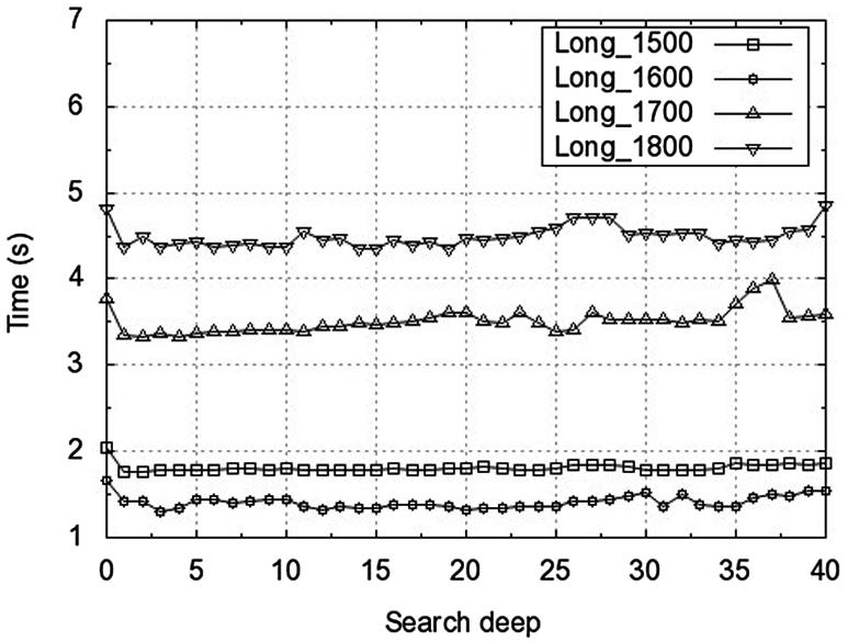
    *Fig 4: Relationship of search depth and search time relative to obstacle length.*

    ## Critical Analysis & Conclusion
    ### Takeaway
    The ASPO approach successfully shifts shortest-path discovery from a static graph problem to a dynamic, obstacle-aware optimization task. By refining the Manhattan distance heuristic, the authors provide a practical tool for real-world LBS apps where "the shortest path" can change by the minute.

    ### Limitations
    While effective in a 2D grid, the paper focuses primarily on static obstacles that enter "temporarily." In a truly high-mobility social network, obstacles (like other users or moving vehicles) might be dynamic. The current model might require even more frequent updates to handle high-velocity moving targets.

    ### Future Work
    The next step for this research lineage would be integrating **Real-time Social Signals** into the weight $w_{i,j}$ of the edges—using data from other users to "predict" where obstacles will appear before the search agent even reaches them.